.ipynb .pdf

Contents

Interactivity with napari

Spatialproteomics has a variety of functions to ensure interoperability with existing tools. For example, we can export the spatialproteomics object into spatialdata, and the use napari for interactive visualizations.

import spatialproteomics as sp
import xarray as xr
from napari_spatialdata import Interactive
import numpy as np

# loading in a data set and performing some formatting for convenience
ds = xr.open_zarr("../../data/LN_11_1.zarr")
ds

<xarray.Dataset> Size: 7GB
Dimensions:            (cells: 16871, cells_2: 16871, channels: 56, y: 3000,
                        x: 3000, la_features: 4, labels: 18, la_props: 2,
                        neighborhoods: 6, nh_props: 2, features: 22)
Coordinates:
  * cells              (cells) int64 135kB 1 2 3 4 5 ... 16868 16869 16870 16871
  * cells_2            (cells_2) int64 135kB 1 2 3 4 ... 16868 16869 16870 16871
  * channels           (channels) <U11 2kB 'DAPI' 'Helios' ... 'CD79a' 'Ki-67'
  * features           (features) object 176B 'BCL-2_binarized' ... 'inter_la...
  * la_features        (la_features) object 32B 'labels_0' ... 'labels_3'
  * la_props           (la_props) <U6 48B '_color' '_name'
  * labels             (labels) int64 144B 1 2 3 4 5 6 7 ... 13 14 15 16 17 18
  * neighborhoods      (neighborhoods) int64 48B 1 2 3 4 5 6
  * nh_props           (nh_props) <U6 48B '_color' '_name'
  * x                  (x) int64 24kB 0 1 2 3 4 5 ... 2995 2996 2997 2998 2999
  * y                  (y) int64 24kB 0 1 2 3 4 5 ... 2995 2996 2997 2998 2999
Data variables:
    _adjacency_matrix  (cells, cells_2) int64 2GB dask.array<chunksize=(528, 528), meta=np.ndarray>
    _image             (channels, y, x) float64 4GB dask.array<chunksize=(4, 375, 375), meta=np.ndarray>
    _image_raw         (channels, y, x) uint8 504MB dask.array<chunksize=(7, 375, 750), meta=np.ndarray>
    _intensity         (cells, channels) float64 8MB dask.array<chunksize=(4218, 14), meta=np.ndarray>
    _la_layers         (cells, la_features) object 540kB dask.array<chunksize=(8436, 4), meta=np.ndarray>
    _la_properties     (labels, la_props) object 288B dask.array<chunksize=(18, 2), meta=np.ndarray>
    _neighborhoods     (cells, labels) float64 2MB dask.array<chunksize=(4218, 9), meta=np.ndarray>
    _nh_properties     (neighborhoods, nh_props) <U14 672B dask.array<chunksize=(6, 2), meta=np.ndarray>
    _obs               (cells, features) float64 3MB dask.array<chunksize=(4218, 11), meta=np.ndarray>
    _segmentation      (y, x) int64 72MB dask.array<chunksize=(375, 375), meta=np.ndarray>

xarray.Dataset

• Dimensions:
  • cells: 16871
  • cells_2: 16871
  • channels: 56
  • y: 3000
  • x: 3000
  • la_features: 4
  • labels: 18
  • la_props: 2
  • neighborhoods: 6
  • nh_props: 2
  • features: 22
• Coordinates: (11)
  • cells
    (cells)
    int64
    1 2 3 4 ... 16868 16869 16870 16871

    array([    1,     2,     3, ..., 16869, 16870, 16871])

  • cells_2
    (cells_2)
    int64
    1 2 3 4 ... 16868 16869 16870 16871

    array([    1,     2,     3, ..., 16869, 16870, 16871])

  • channels
    (channels)
    <U11
    'DAPI' 'Helios' ... 'CD79a' 'Ki-67'

    array(['DAPI', 'Helios', 'CD10', 'TCF7/TCF1', 'PD-L1', 'BCL-6', 'FOXP3',
           'CD69', 'Perforin', 'CD19', 'LAG3', 'CD21', 'CD62L', 'c-myc', 'CD138',
           'CD15', 'BCL-2', 'CD56', 'IKZF3', 'CD25', 'NOXA', 'Tim3', 'Serpin B9',
           'Podoplanin', 'CD38', 'SPARC', 'ICOS', 'CXCR5', 'CD163', 'FADD', 'p53',
           'Collagen IV', 'CD4', 'CD7', 'Kappa', 'CD20', 'CD34', 'PAX5', 'PD-1',
           'CD45RA', 'CD11b', 'Lambda', 'CD57', 'CD11c', 'CD90', 'HLA DR', 'CD68',
           'CD31', 'CD45', 'CD3', 'Cytokeratin', 'CD45RO', 'CD8', 'Granzyme B',
           'CD79a', 'Ki-67'], dtype='<U11')

  • features
    (features)
    object
    'BCL-2_binarized' ... 'inter_lab...

    array(['BCL-2_binarized', 'BCL-6_binarized', 'CD163_binarized',
           'CD45RA_binarized', 'CD45RO_binarized', 'CD8_binarized',
           'DAPI_binarized', 'FOXP3_binarized', 'Helios_binarized',
           'ICOS_binarized', 'Ki-67_binarized', 'PD-1_binarized',
           'TCF7-TCF1_binarized', 'Tim3_binarized', '_labels', '_neighborhoods',
           'centroid-0', 'centroid-1', 'degree', 'diversity_index', 'homophily',
           'inter_label_connectivity'], dtype=object)

  • la_features
    (la_features)
    object
    'labels_0' ... 'labels_3'

    array(['labels_0', 'labels_1', 'labels_2', 'labels_3'], dtype=object)

  • la_props
    (la_props)
    <U6
    '_color' '_name'

    array(['_color', '_name'], dtype='<U6')

  • labels
    (labels)
    int64
    1 2 3 4 5 6 7 ... 13 14 15 16 17 18

    array([ 1,  2,  3,  4,  5,  6,  7,  8,  9, 10, 11, 12, 13, 14, 15, 16, 17, 18])

  • neighborhoods
    (neighborhoods)
    int64
    1 2 3 4 5 6

    array([1, 2, 3, 4, 5, 6])

  • nh_props
    (nh_props)
    <U6
    '_color' '_name'

    array(['_color', '_name'], dtype='<U6')

  • x
    (x)
    int64
    0 1 2 3 4 ... 2996 2997 2998 2999

    array([   0,    1,    2, ..., 2997, 2998, 2999])

  • y
    (y)
    int64
    0 1 2 3 4 ... 2996 2997 2998 2999

    array([   0,    1,    2, ..., 2997, 2998, 2999])

• Data variables: (10)
  • _adjacency_matrix
    (cells, cells_2)
    int64
    dask.array<chunksize=(528, 528), meta=np.ndarray>

    Array Chunk Bytes 2.12 GiB 2.13 MiB Shape (16871, 16871) (528, 528) Dask graph 1024 chunks in 2 graph layers Data type int64 numpy.ndarray

  • _image
    (channels, y, x)
    float64
    dask.array<chunksize=(4, 375, 375), meta=np.ndarray>

    Array Chunk Bytes 3.76 GiB 4.29 MiB Shape (56, 3000, 3000) (4, 375, 375) Dask graph 896 chunks in 2 graph layers Data type float64 numpy.ndarray

  • _image_raw
    (channels, y, x)
    uint8
    dask.array<chunksize=(7, 375, 750), meta=np.ndarray>

    Array Chunk Bytes 480.65 MiB 1.88 MiB Shape (56, 3000, 3000) (7, 375, 750) Dask graph 256 chunks in 2 graph layers Data type uint8 numpy.ndarray

  • _intensity
    (cells, channels)
    float64
    dask.array<chunksize=(4218, 14), meta=np.ndarray>

    Array Chunk Bytes 7.21 MiB 461.34 kiB Shape (16871, 56) (4218, 14) Dask graph 16 chunks in 2 graph layers Data type float64 numpy.ndarray

  • _la_layers
    (cells, la_features)
    object
    dask.array<chunksize=(8436, 4), meta=np.ndarray>

    Array Chunk Bytes 527.22 kiB 263.62 kiB Shape (16871, 4) (8436, 4) Dask graph 2 chunks in 2 graph layers Data type object numpy.ndarray

  • _la_properties
    (labels, la_props)
    object
    dask.array<chunksize=(18, 2), meta=np.ndarray>

    Array Chunk Bytes 288 B 288 B Shape (18, 2) (18, 2) Dask graph 1 chunks in 2 graph layers Data type object numpy.ndarray

  • _neighborhoods
    (cells, labels)
    float64
    dask.array<chunksize=(4218, 9), meta=np.ndarray>

    Array Chunk Bytes 2.32 MiB 296.58 kiB Shape (16871, 18) (4218, 9) Dask graph 8 chunks in 2 graph layers Data type float64 numpy.ndarray

  • _nh_properties
    (neighborhoods, nh_props)
    <U14
    dask.array<chunksize=(6, 2), meta=np.ndarray>

    Array Chunk Bytes 672 B 672 B Shape (6, 2) (6, 2) Dask graph 1 chunks in 2 graph layers Data type

  • _obs
    (cells, features)
    float64
    dask.array<chunksize=(4218, 11), meta=np.ndarray>

    Array Chunk Bytes 2.83 MiB 362.48 kiB Shape (16871, 22) (4218, 11) Dask graph 8 chunks in 2 graph layers Data type float64 numpy.ndarray

  • _segmentation
    (y, x)
    int64
    dask.array<chunksize=(375, 375), meta=np.ndarray>

    Array Chunk Bytes 68.66 MiB 1.07 MiB Shape (3000, 3000) (375, 375) Dask graph 64 chunks in 2 graph layers Data type int64 numpy.ndarray

• Indexes: (11)
  • cells
    PandasIndex

    PandasIndex(Index([    1,     2,     3,     4,     5,     6,     7,     8,     9,    10,
           ...
           16862, 16863, 16864, 16865, 16866, 16867, 16868, 16869, 16870, 16871],
          dtype='int64', name='cells', length=16871))

  • cells_2
    PandasIndex

    PandasIndex(Index([    1,     2,     3,     4,     5,     6,     7,     8,     9,    10,
           ...
           16862, 16863, 16864, 16865, 16866, 16867, 16868, 16869, 16870, 16871],
          dtype='int64', name='cells_2', length=16871))

  • channels
    PandasIndex

    PandasIndex(Index(['DAPI', 'Helios', 'CD10', 'TCF7/TCF1', 'PD-L1', 'BCL-6', 'FOXP3',
           'CD69', 'Perforin', 'CD19', 'LAG3', 'CD21', 'CD62L', 'c-myc', 'CD138',
           'CD15', 'BCL-2', 'CD56', 'IKZF3', 'CD25', 'NOXA', 'Tim3', 'Serpin B9',
           'Podoplanin', 'CD38', 'SPARC', 'ICOS', 'CXCR5', 'CD163', 'FADD', 'p53',
           'Collagen IV', 'CD4', 'CD7', 'Kappa', 'CD20', 'CD34', 'PAX5', 'PD-1',
           'CD45RA', 'CD11b', 'Lambda', 'CD57', 'CD11c', 'CD90', 'HLA DR', 'CD68',
           'CD31', 'CD45', 'CD3', 'Cytokeratin', 'CD45RO', 'CD8', 'Granzyme B',
           'CD79a', 'Ki-67'],
          dtype='object', name='channels'))

  • features
    PandasIndex

    PandasIndex(Index(['BCL-2_binarized', 'BCL-6_binarized', 'CD163_binarized',
           'CD45RA_binarized', 'CD45RO_binarized', 'CD8_binarized',
           'DAPI_binarized', 'FOXP3_binarized', 'Helios_binarized',
           'ICOS_binarized', 'Ki-67_binarized', 'PD-1_binarized',
           'TCF7-TCF1_binarized', 'Tim3_binarized', '_labels', '_neighborhoods',
           'centroid-0', 'centroid-1', 'degree', 'diversity_index', 'homophily',
           'inter_label_connectivity'],
          dtype='object', name='features'))

  • la_features
    PandasIndex

    PandasIndex(Index(['labels_0', 'labels_1', 'labels_2', 'labels_3'], dtype='object', name='la_features'))

  • la_props
    PandasIndex

    PandasIndex(Index(['_color', '_name'], dtype='object', name='la_props'))

  • labels
    PandasIndex

    PandasIndex(Index([1, 2, 3, 4, 5, 6, 7, 8, 9, 10, 11, 12, 13, 14, 15, 16, 17, 18], dtype='int64', name='labels'))

  • neighborhoods
    PandasIndex

    PandasIndex(Index([1, 2, 3, 4, 5, 6], dtype='int64', name='neighborhoods'))

  • nh_props
    PandasIndex

    PandasIndex(Index(['_color', '_name'], dtype='object', name='nh_props'))

  • x
    PandasIndex

    PandasIndex(Index([   0,    1,    2,    3,    4,    5,    6,    7,    8,    9,
           ...
           2990, 2991, 2992, 2993, 2994, 2995, 2996, 2997, 2998, 2999],
          dtype='int64', name='x', length=3000))

  • y
    PandasIndex

    PandasIndex(Index([   0,    1,    2,    3,    4,    5,    6,    7,    8,    9,
           ...
           2990, 2991, 2992, 2993, 2994, 2995, 2996, 2997, 2998, 2999],
          dtype='int64', name='y', length=3000))

• Attributes: (0)

# turning the spatialproteomics object into a spatialdata object
sd_obj = ds.tl.convert_to_spatialdata()
sd_obj

INFO     Transposing `data` of type: <class 'dask.array.core.Array'> to ('c', 'y', 'x').
INFO     Transposing `data` of type: <class 'dask.array.core.Array'> to ('y', 'x').

SpatialData object
├── Images
│     └── 'image': DataArray[cyx] (56, 3000, 3000)
├── Labels
│     └── 'segmentation': DataArray[yx] (3000, 3000)
└── Tables
      └── 'table': AnnData (16871, 56)
with coordinate systems:
    ▸ 'global', with elements:
        image (Images), segmentation (Labels)

interactive = Interactive(sd_obj)
interactive.run()

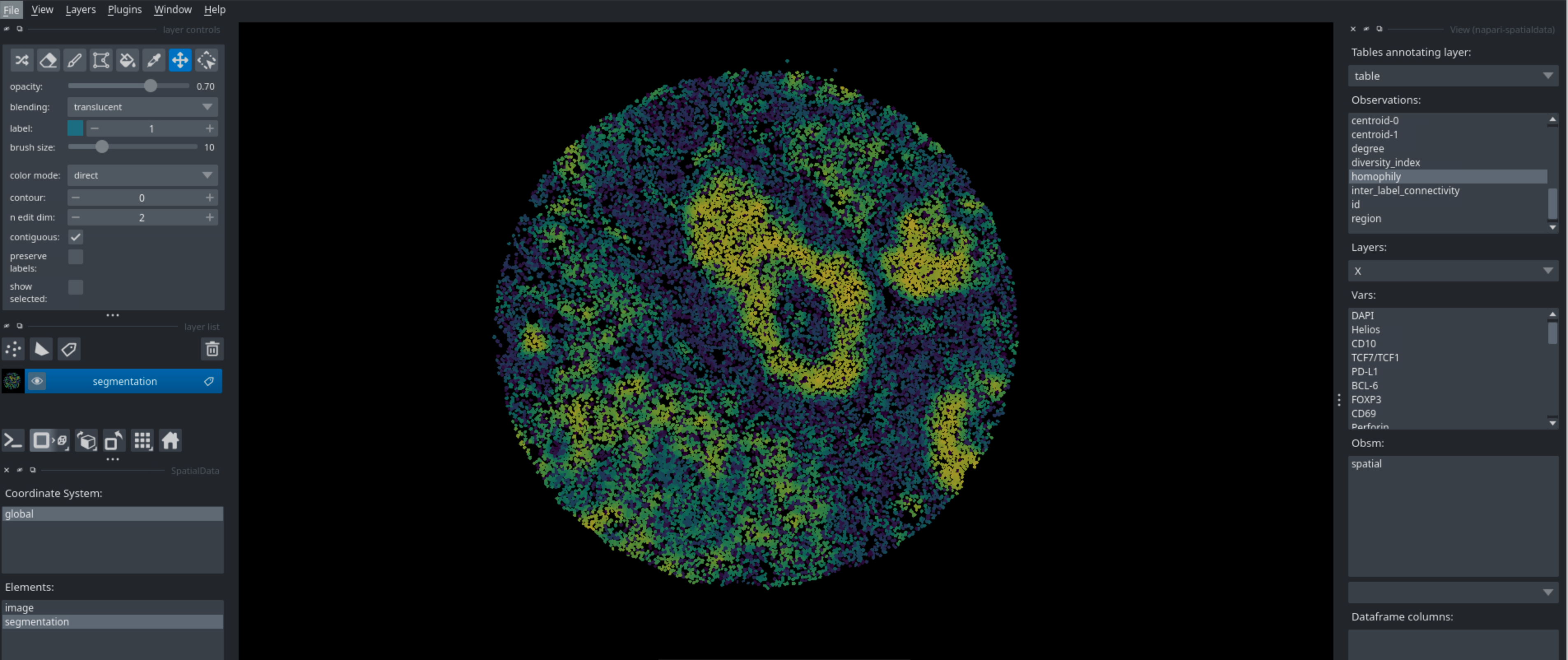
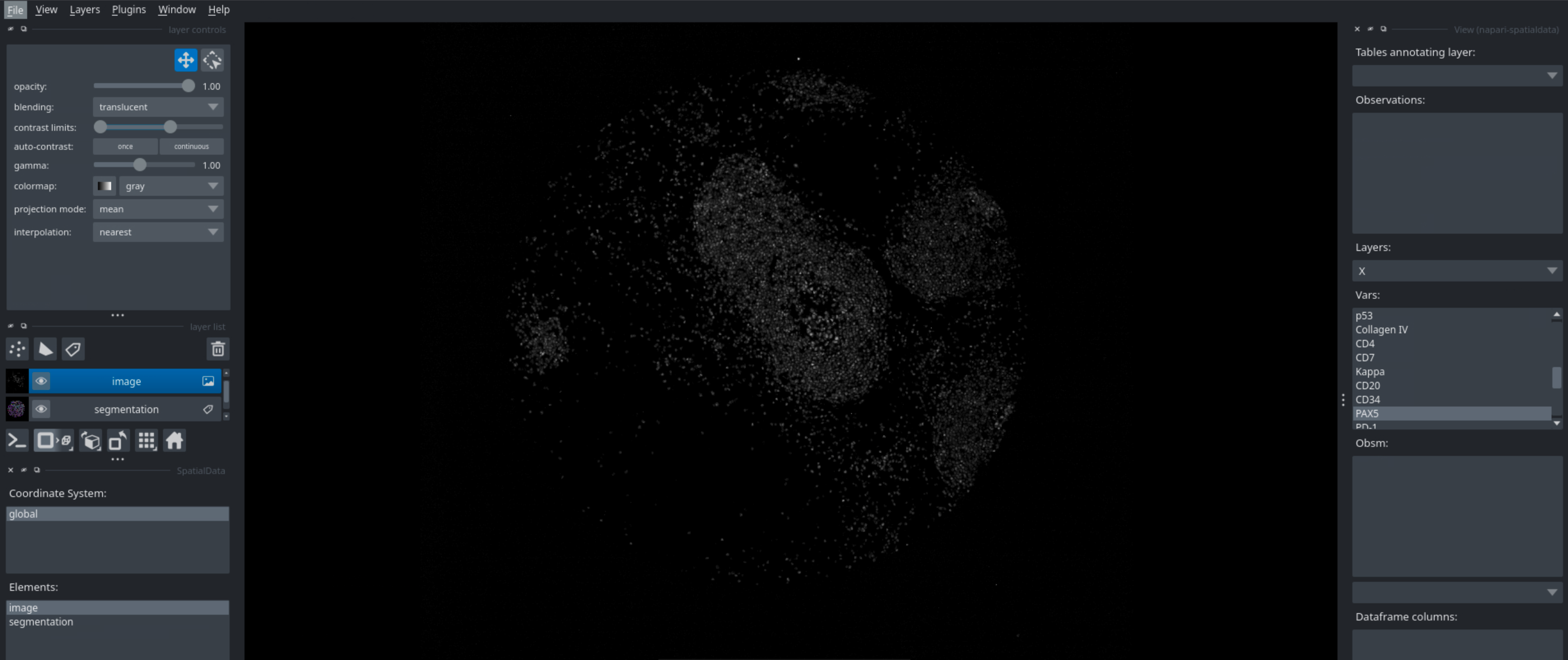
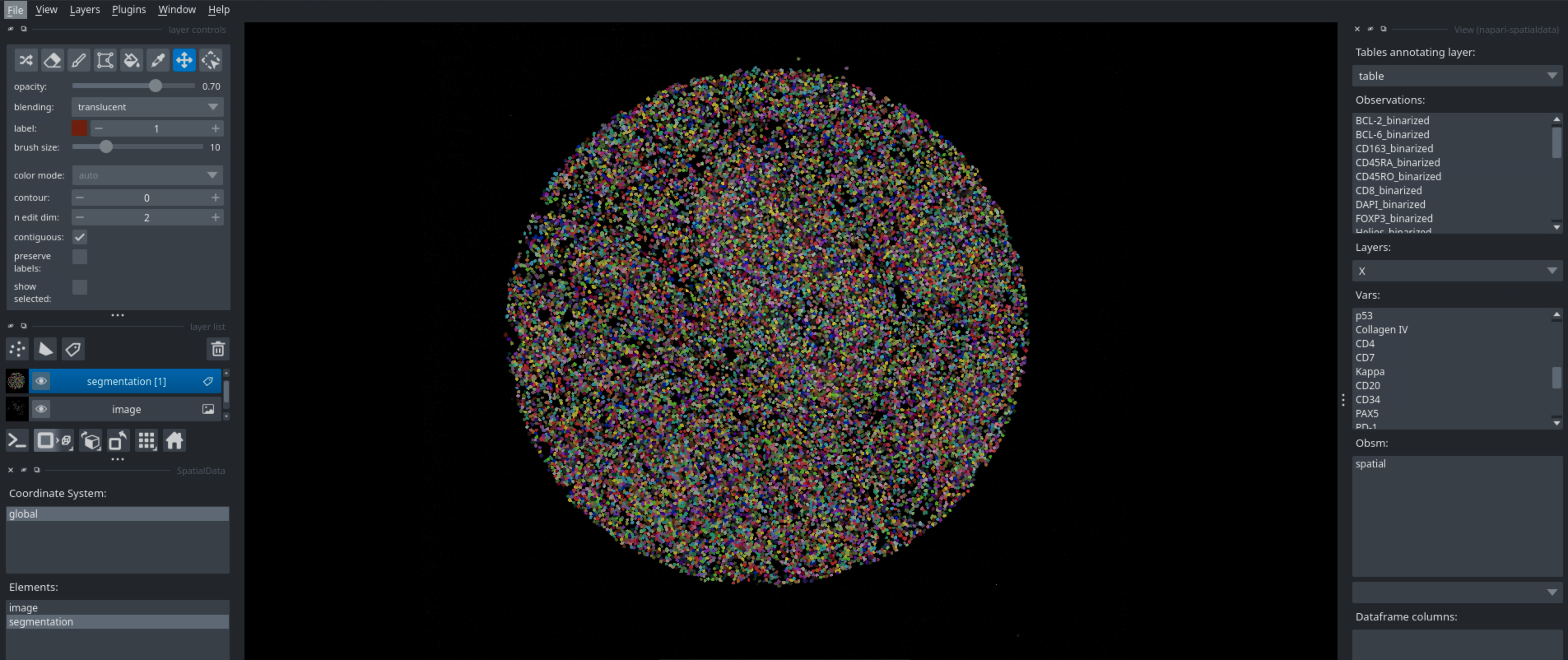
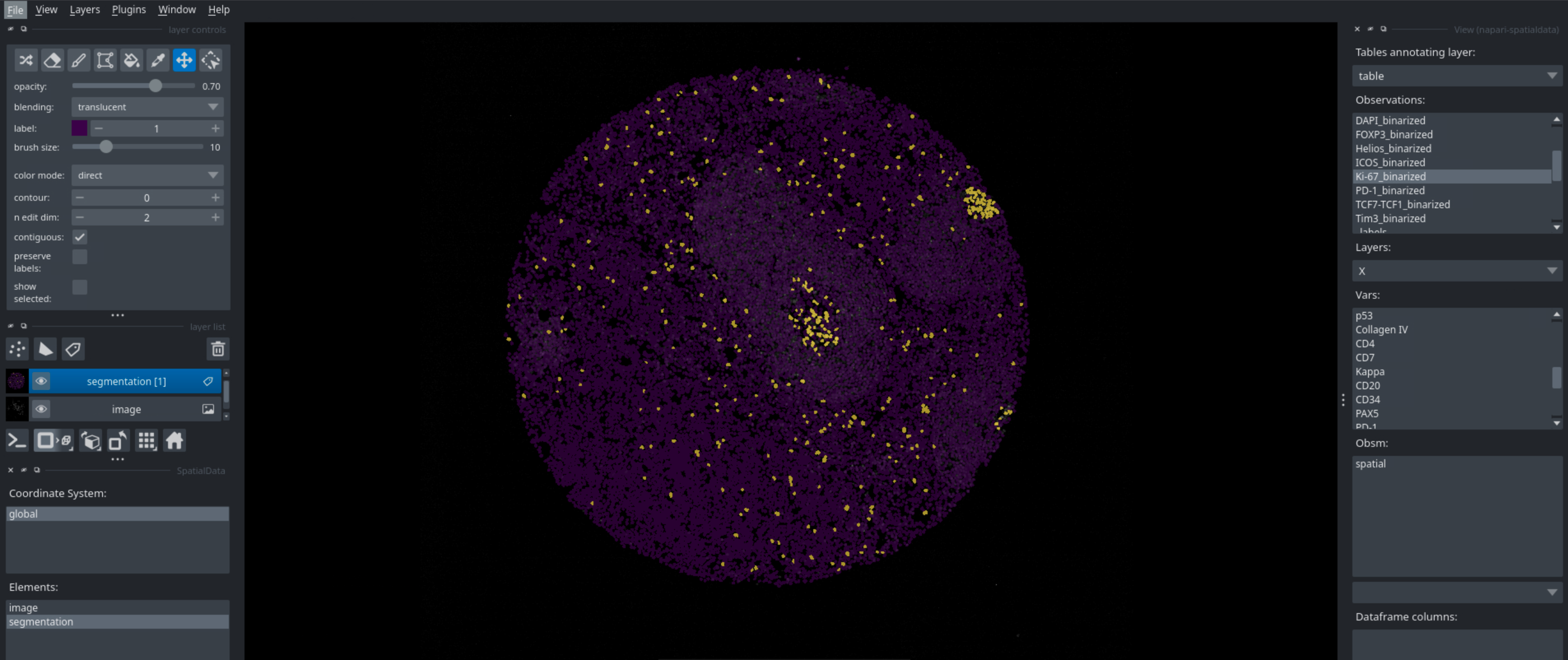
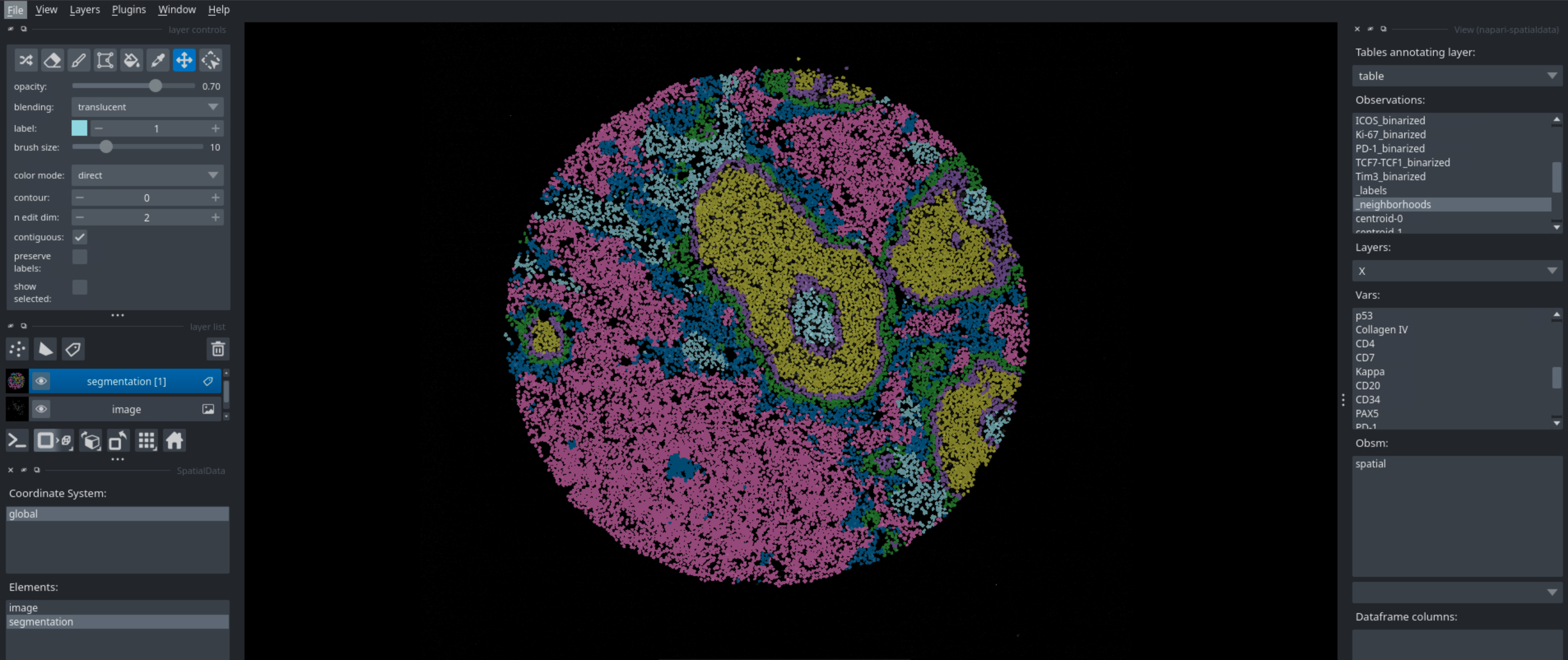
Running this code in a python script will open napari, which you can then use to interactively look at your data. You can look at different markers, visualize cell types, neighborhoods, and many more. Below are some examples of what you can visualize with napari.

Markers

Segmentation

Cell Type Labels

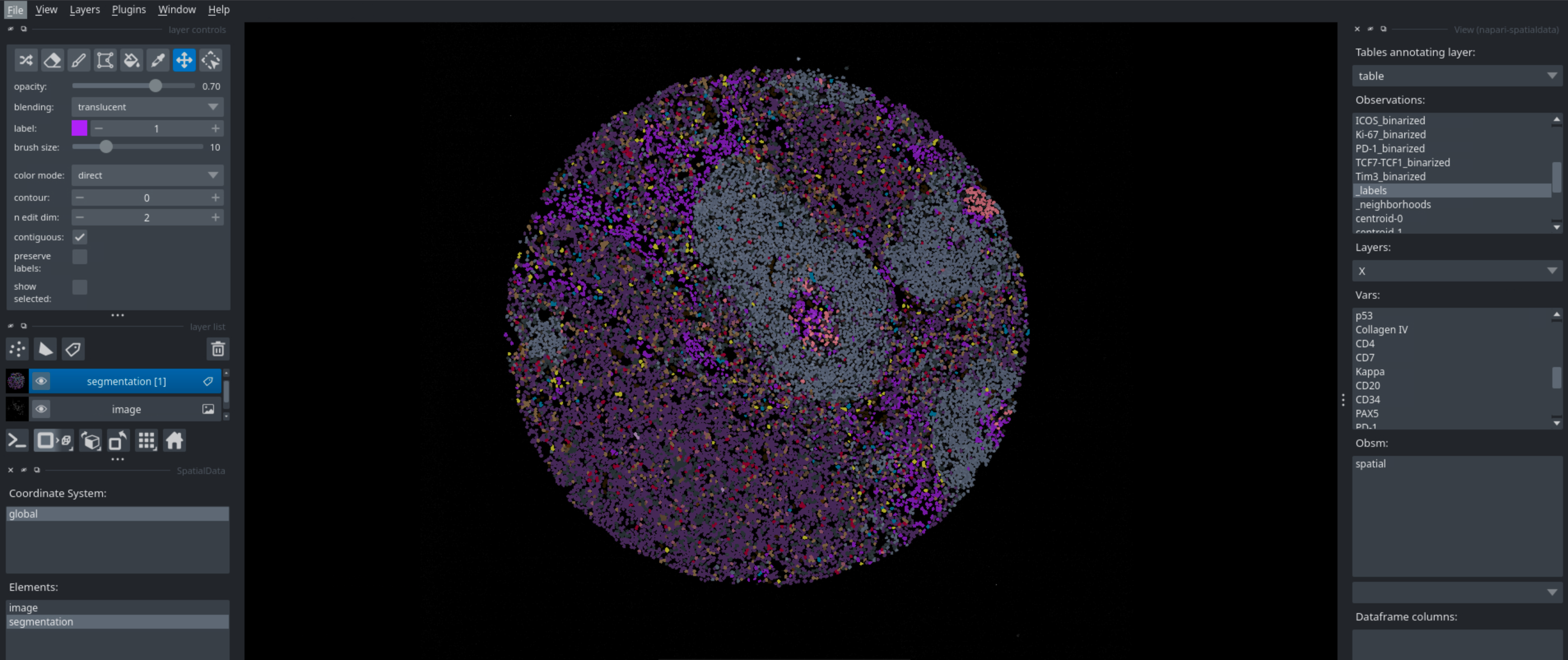
Binarization

Neighborhoods

Features

Downstream Analysis Customizability